D^+\to\pi^+\pi^+\pi^- with Dalitz-plot decomposition

\(D^+\to\pi^+\pi^+\pi^-\) with Dalitz-plot decomposition#

This report demonstrates a Bose-symmetric isobar model for \(D^+\to\pi^+\pi^+\pi^-\) using QRules for transition generation, AmpForm-DPD for symbolic helicity amplitudes, and TensorWaves for numerical evaluation. The amplitude is checked for Bose symmetry and used to plot an illustrative Dalitz density.

The resonance content follows two published analyses:

CLEO [Bonvicini and others, 2007], Table II: \(\rho(770)\), \(f_2(1270)\), \(f_0(980)\), \(f_0(1370)\), \(f_0(1500)\), and a low-mass \(\sigma\) component, represented here by \(f_0(500)\).
LHCb [Aaij and others, 2023], Table 2: also includes \(\omega(782)\), \(\rho(1450)\), and \(\rho(1700)\). Its S wave is determined with a quasi-model-independent parametrization, rather than separate scalar isobars. States tested without significant improvement, such as \(\rho_3(1690)\), are not included here.

This nine-resonance example combines CLEO’s scalar-isobar content with the additional LHCb vector states. It retains the package Breit–Wigner dynamics, masses, widths, and radii. CLEO instead uses a complex \(\sigma\) pole and a Flatté function for \(f_0(980)\); LHCb uses Gounaris–Sakurai functions for the \(\rho\) states. The S wave, especially near the \(K\bar K\) threshold, therefore remains an approximation. The source fit-fraction ratios set the relative component strengths below; the result is a literature-informed illustration, not a reproduction of either fit. No CP violation is assumed.

Generate the decay chains#

Label \(D^+\) by 0 and \((\pi^+_1,\pi^+_2,\pi^-_3)\) by \((1,2,3)\). The charm decay is weak, so imposing strong-interaction conservation on the entire chain would incorrectly forbid it. We allow weak interactions in QRules; the selected neutral resonances also have strong-decay-compatible \(J^P\) for their two-pion daughters.

qrules: 0.10.12
ampform-dpd: 0.2.4
tensorwaves: 0.4.17

resonance	\(J^P\)	mass (MeV)	width (MeV)	\(L_\mathrm{dec}^\mathrm{min}\)	\(L_\mathrm{prod}^\mathrm{min}\)
\(f_{0}(1370) \to \pi^{+} \pi^{-}\)	\(0^+\)	1,350	350	0	0
\(f_{0}(1500) \to \pi^{+} \pi^{-}\)	\(0^+\)	1,522	108	0	0
\(f_{0}(500) \to \pi^{+} \pi^{-}\)	\(0^+\)	600	450	0	0
\(f_{0}(980) \to \pi^{+} \pi^{-}\)	\(0^+\)	990	60	0	0
\(f_{2}(1270) \to \pi^{+} \pi^{-}\)	\(2^+\)	1,275	186	2	2
\(\omega(782) \to \pi^{+} \pi^{-}\)	\(1^-\)	782	8	1	1
\(\rho(1450)^{0} \to \pi^{+} \pi^{-}\)	\(1^-\)	1,465	400	1	1
\(\rho(1700)^{0} \to \pi^{+} \pi^{-}\)	\(1^-\)	1,720	250	1	1
\(\rho(770)^{0} \to \pi^{+} \pi^{-}\)	\(1^-\)	775	147	1	1

Formulate and display the model#

Define

\[s=\sigma_1=(p_2+p_3)^2,\qquad t=\sigma_2=(p_1+p_3)^2,\qquad u=\sigma_3=(p_1+p_2)^2,\]

The invariant relation, scattering angle, and dynamics definitions below are rendered from the model and package expression objects. All external spins are zero, so the Wigner functions reduce to Legendre polynomials.

The dynamics factor \(X_R\) is the product of the resonance lineshape and the production and decay form factors. \(B_J^2\) is AmpForm’s normalized Blatt–Weisskopf function, with \(B_J^2(1)=1\). Both radii retain the package default of \(1\,\mathrm{GeV}^{-1}\). Angular momentum requires \(L_\mathrm{production}=L_\mathrm{decay}=J_R\); canonical-helicity supplies these orbital angular momenta to the dynamics builder.

The installed AmpForm-DPD v0.2.4 builder passes \(s^2\) to the decay form factor and the pole mass \(m_R\) as a production daughter mass. The correction below replaces these arguments by \(s\) and \(\sqrt{s}\), respectively. The Breit–Wigner, running width, and form-factor implementations remain those of the packages.

The Bose-symmetric amplitude and intensity are

\[\mathcal A(s,t)=\sum_R c_R\left[X_R(s)P_{J_R}(z(s,t))+X_R(t)P_{J_R}(z(t,s))\right],\qquad I(s,t)=|\mathcal A(s,t)|^2,\]

AmpForm’s HelicityAmplitudeBuilder includes identical-particle symmetrization automatically; the fix for this channel was released in v0.15.9 (see the accepted answer in discussion #475). This report uses DalitzPlotDecompositionBuilder from AmpForm-DPD instead.

In AmpForm-DPD v0.2.4, permute_equal_final_states generates both particle assignments, but their helicity couplings must account for the daughter-order convention. Writing \(z(s,t)=\cos\theta_{23}\), for equal pion masses the generated angles satisfy \(\cos\theta_{31}(s,t)=-z(t,s)\). Consequently, \(P_J(-z)=(-1)^J P_J(z)\) introduces a relative minus sign for the P wave if the two subsystems are summed with unchanged helicity couplings. Here we formulate subsystem 1 and explicitly exchange \(s\leftrightarrow t\) in its amplitude, retaining the same complex coefficient and daughter convention. The complex-amplitude symmetry check below verifies this construction.

An overall \(1/\sqrt{2!}\) amplitude convention is absorbed into normalization. The plot covers the full labelled Dalitz domain; integration for an absolute identical-particle rate requires the corresponding \(1/2!\) phase-space factor.

s, t, u = sp.symbols("sigma1:4", nonnegative=True)
m0, m1, m2, m3 = sp.symbols("m:4", nonnegative=True)

builder = DalitzPlotDecompositionBuilder(decay)
for name in resonance_names:
    builder.dynamics_choices.register_builder(
        name, formulate_breit_wigner_with_form_factor
    )
model = builder.formulate(cleanup_summations=True, use_coefficients=True)
assert len(model.amplitudes) == 1

# Correct form-factor kinematics in AmpForm-DPD v0.2.4.
form_factor_corrections = {}
for expression in model.amplitudes.values():
    for ff in expression.atoms(FormFactor):
        if ff.s == s**2:
            form_factor_corrections[ff] = FormFactor(
                s, ff.m1, ff.m2, ff.angular_momentum, ff.meson_radius
            )
        elif ff.s == m0**2:
            form_factor_corrections[ff] = FormFactor(
                m0**2, sp.sqrt(s), ff.m2, ff.angular_momentum, ff.meson_radius
            )
model.amplitudes.update({
    symbol: expression.xreplace(form_factor_corrections)
    for symbol, expression in model.amplitudes.items()
})
Math(aslatex(model.amplitudes, terms_per_line=1))

\[\begin{split}\displaystyle \begin{aligned} {A^{1}}_{0,0,0,0} \;&=\; \sum_{\lambda_{R}=0}{\delta_{0 \lambda_{R}} \mathcal{F}_{0}\left(m_{0}^{2}, \sqrt{\sigma_{1}}, m_{\pi^{+}}\right) \mathcal{F}_{0}\left(\sigma_{1}, m_{\pi^{+}}, m_{\pi^{-}}\right) {\mathcal{H}^\mathrm{f_{0}(1370)}}_{\lambda_{R},0,0,0} \mathcal{R}_{0}\left(\sigma_{1}, m_{f_{0}(1370)}, \Gamma_{f_{0}(1370)}\right) d^{0}_{\lambda_{R},0}\left(\theta_{23}\right)} \\ \;&+\; \sum_{\lambda_{R}=0}{\delta_{0 \lambda_{R}} \mathcal{F}_{0}\left(m_{0}^{2}, \sqrt{\sigma_{1}}, m_{\pi^{+}}\right) \mathcal{F}_{0}\left(\sigma_{1}, m_{\pi^{+}}, m_{\pi^{-}}\right) {\mathcal{H}^\mathrm{f_{0}(1500)}}_{\lambda_{R},0,0,0} \mathcal{R}_{0}\left(\sigma_{1}, m_{f_{0}(1500)}, \Gamma_{f_{0}(1500)}\right) d^{0}_{\lambda_{R},0}\left(\theta_{23}\right)} \\ \;&+\; \sum_{\lambda_{R}=0}{\delta_{0 \lambda_{R}} \mathcal{F}_{0}\left(m_{0}^{2}, \sqrt{\sigma_{1}}, m_{\pi^{+}}\right) \mathcal{F}_{0}\left(\sigma_{1}, m_{\pi^{+}}, m_{\pi^{-}}\right) {\mathcal{H}^\mathrm{f_{0}(500)}}_{\lambda_{R},0,0,0} \mathcal{R}_{0}\left(\sigma_{1}, m_{f_{0}(500)}, \Gamma_{f_{0}(500)}\right) d^{0}_{\lambda_{R},0}\left(\theta_{23}\right)} \\ \;&+\; \sum_{\lambda_{R}=0}{\delta_{0 \lambda_{R}} \mathcal{F}_{0}\left(m_{0}^{2}, \sqrt{\sigma_{1}}, m_{\pi^{+}}\right) \mathcal{F}_{0}\left(\sigma_{1}, m_{\pi^{+}}, m_{\pi^{-}}\right) {\mathcal{H}^\mathrm{f_{0}(980)}}_{\lambda_{R},0,0,0} \mathcal{R}_{0}\left(\sigma_{1}, m_{f_{0}(980)}, \Gamma_{f_{0}(980)}\right) d^{0}_{\lambda_{R},0}\left(\theta_{23}\right)} \\ \;&+\; \sum_{\lambda_{R}=-1}^{1}{\delta_{0 \lambda_{R}} \mathcal{F}_{1}\left(m_{0}^{2}, \sqrt{\sigma_{1}}, m_{\pi^{+}}\right) \mathcal{F}_{1}\left(\sigma_{1}, m_{\pi^{+}}, m_{\pi^{-}}\right) {\mathcal{H}^\mathrm{\omega(782)}}_{\lambda_{R},0,0,0} \mathcal{R}_{1}\left(\sigma_{1}, m_{\omega(782)}, \Gamma_{\omega(782)}\right) d^{1}_{\lambda_{R},0}\left(\theta_{23}\right)} \\ \;&+\; \sum_{\lambda_{R}=-1}^{1}{\delta_{0 \lambda_{R}} \mathcal{F}_{1}\left(m_{0}^{2}, \sqrt{\sigma_{1}}, m_{\pi^{+}}\right) \mathcal{F}_{1}\left(\sigma_{1}, m_{\pi^{+}}, m_{\pi^{-}}\right) {\mathcal{H}^\mathrm{\rho(1450)^{0}}}_{\lambda_{R},0,0,0} \mathcal{R}_{1}\left(\sigma_{1}, m_{\rho(1450)^{0}}, \Gamma_{\rho(1450)^{0}}\right) d^{1}_{\lambda_{R},0}\left(\theta_{23}\right)} \\ \;&+\; \sum_{\lambda_{R}=-1}^{1}{\delta_{0 \lambda_{R}} \mathcal{F}_{1}\left(m_{0}^{2}, \sqrt{\sigma_{1}}, m_{\pi^{+}}\right) \mathcal{F}_{1}\left(\sigma_{1}, m_{\pi^{+}}, m_{\pi^{-}}\right) {\mathcal{H}^\mathrm{\rho(1700)^{0}}}_{\lambda_{R},0,0,0} \mathcal{R}_{1}\left(\sigma_{1}, m_{\rho(1700)^{0}}, \Gamma_{\rho(1700)^{0}}\right) d^{1}_{\lambda_{R},0}\left(\theta_{23}\right)} \\ \;&+\; \sum_{\lambda_{R}=-1}^{1}{\delta_{0 \lambda_{R}} \mathcal{F}_{1}\left(m_{0}^{2}, \sqrt{\sigma_{1}}, m_{\pi^{+}}\right) \mathcal{F}_{1}\left(\sigma_{1}, m_{\pi^{+}}, m_{\pi^{-}}\right) {\mathcal{H}^\mathrm{\rho(770)^{0}}}_{\lambda_{R},0,0,0} \mathcal{R}_{1}\left(\sigma_{1}, m_{\rho(770)^{0}}, \Gamma_{\rho(770)^{0}}\right) d^{1}_{\lambda_{R},0}\left(\theta_{23}\right)} \\ \;&+\; \sum_{\lambda_{R}=-2}^{2}{\delta_{0 \lambda_{R}} \mathcal{F}_{2}\left(m_{0}^{2}, \sqrt{\sigma_{1}}, m_{\pi^{+}}\right) \mathcal{F}_{2}\left(\sigma_{1}, m_{\pi^{+}}, m_{\pi^{-}}\right) {\mathcal{H}^\mathrm{f_{2}(1270)}}_{\lambda_{R},0,0,0} \mathcal{R}_{2}\left(\sigma_{1}, m_{f_{2}(1270)}, \Gamma_{f_{2}(1270)}\right) d^{2}_{\lambda_{R},0}\left(\theta_{23}\right)} \\ \end{aligned}\end{split}\]

The kinematic definitions and spin factors are

\[\begin{split}\displaystyle \begin{aligned} \sigma_{3} \;&=\; m_{0}^{2} + m_{1}^{2} + m_{2}^{2} + m_{3}^{2} - \sigma_{1} - \sigma_{2} \\ \lambda\left(x, y, z\right) \;&=\; x^{2} - 2 x y - 2 x z + y^{2} - 2 y z + z^{2} \\ \theta_{23} \;&=\; \operatorname{acos}{\left(\frac{2 \sigma_{1} \left(- m_{1}^{2} - m_{2}^{2} + \sigma_{3}\right) - \left(m_{0}^{2} - m_{1}^{2} - \sigma_{1}\right) \left(m_{2}^{2} - m_{3}^{2} + \sigma_{1}\right)}{\sqrt{\lambda\left(m_{0}^{2}, m_{1}^{2}, \sigma_{1}\right)} \sqrt{\lambda\left(\sigma_{1}, m_{2}^{2}, m_{3}^{2}\right)}} \right)} \\ d^{0}_{0,0}\left(\operatorname{acos}{\left(z \right)}\right) \;&=\; 1 \\ d^{1}_{0,0}\left(\operatorname{acos}{\left(z \right)}\right) \;&=\; z \\ d^{2}_{0,0}\left(\operatorname{acos}{\left(z \right)}\right) \;&=\; \frac{3 z^{2}}{2} - \frac{1}{2} \\ \end{aligned}\end{split}\]

The tensor-wave lineshape illustrates the package dynamics. Each definition is obtained by evaluating one layer of its expression object; the barrier factors are shown for all three spins.

\[\begin{split}\displaystyle \begin{aligned} X_{f_{2}(1270)}{\left(\sigma_{1} \right)} \;&=\; \mathcal{F}_{2}\left(m_{0}^{2}, \sqrt{\sigma_{1}}, m_{\pi^{+}}\right) \mathcal{F}_{2}\left(\sigma_{1}, m_{\pi^{+}}, m_{\pi^{-}}\right) \mathcal{R}_{2}\left(\sigma_{1}, m_{f_{2}(1270)}, \Gamma_{f_{2}(1270)}\right) \\ \mathcal{R}_{2}\left(\sigma_{1}, m_{f_{2}(1270)}, \Gamma_{f_{2}(1270)}\right) \;&=\; \frac{\Gamma_{f_{2}(1270)} m_{f_{2}(1270)}}{m_{f_{2}(1270)}^{2} - i m_{f_{2}(1270)} \Gamma_{2}\left(\sigma_{1}\right) - \sigma_{1}} \\ \Gamma_{2}\left(\sigma_{1}\right) \;&=\; \frac{\Gamma_{f_{2}(1270)} \mathcal{F}_{2}\left(\sigma_{1}, m_{\pi^{+}}, m_{\pi^{-}}\right)^{2} \rho_{1}\left(\sigma_{1}\right)}{\mathcal{F}_{2}\left(m_{f_{2}(1270)}^{2}, m_{\pi^{+}}, m_{\pi^{-}}\right)^{2} \rho_{21270}\left(m_{f_{2}(1270)}^{2}\right)} \\ \mathcal{F}_{2}\left(\sigma_{1}, m_{\pi^{+}}, m_{\pi^{-}}\right) \;&=\; \sqrt{B_{2}^2\left(R_\mathrm{res}^{2} q^2_{1}\left(\sigma_{1}\right)\right)} \\ q^2_{1}\left(\sigma_{1}\right) \;&=\; \frac{\left(\sigma_{1} - \left(m_{\pi^{+}} - m_{\pi^{-}}\right)^{2}\right) \left(\sigma_{1} - \left(m_{\pi^{+}} + m_{\pi^{-}}\right)^{2}\right)}{4 \sigma_{1}} \\ B_{0}^2\left(z\right) \;&=\; 1 \\ B_{1}^2\left(z\right) \;&=\; \frac{2 z}{z + 1} \\ B_{2}^2\left(z\right) \;&=\; \frac{13 z^{2}}{z^{2} + 3 z + 9} \\ \end{aligned}\end{split}\]

# Retain the package coefficient names; set their numerical values below.
couplings = {
    symbol: value
    for symbol, value in model.parameter_defaults.items()
    if isinstance(symbol, sp.Indexed)
}
fixed_parameters = {
    symbol: value
    for symbol, value in model.parameter_defaults.items()
    if symbol not in couplings
}

subamplitude = next(iter(model.amplitudes.values())).doit()
subamplitude = subamplitude.xreplace(model.variables).doit()
subamplitude = subamplitude.subs(u, model.invariants[u])
subamplitude = subamplitude.xreplace(fixed_parameters)
# Preserve the daughter convention when exchanging the identical pions.
amplitude = subamplitude + subamplitude.xreplace({s: t, t: s})
intensity = sp.Abs(amplitude) ** 2
intensity_function = create_parametrized_function(intensity, couplings, backend="numpy")
amplitude_function = create_parametrized_function(amplitude, couplings, backend="numpy")

M = decay.states[0].mass
mpi = decay.states[1].mass
sigma_sum = M**2 + 3 * mpi**2

coefficient_symbols = {
    name: next(symbol for symbol in couplings if resonance.latex in str(symbol))
    for name, resonance in resonances.items()
}
assert len(set(coefficient_symbols.values())) == len(resonance_names)
component_functions = {
    name: create_function(amplitude.diff(symbol), backend="numpy")
    for name, symbol in coefficient_symbols.items()
}

Physical Dalitz domain and numerical checks#

For a scalar parent, three-body phase space is constant in \(ds\,dt\) inside the kinematic boundary. Thus \(I(s,t)\) is proportional to the Dalitz density without an additional momentum weight. The bounds below are rendered from the same symbolic expressions used for numerical evaluation.

We evaluate only interior points, where scattering angles are defined. The checks below verify the corrected form-factor arguments, Bose symmetry of the complex amplitude, and finite nonnegative intensity. An intensity-only symmetry check would miss an antisymmetric amplitude.

Define Dalitz boundaries and validate the amplitude

Hide code cell source

# Verify that both vertices use the running invariant mass.
for expression in model.amplitudes.values():
    for ff in expression.atoms(FormFactor):
        assert ff.s in {s, m0**2}
        if ff.s == m0**2:
            assert ff.m1 == sp.sqrt(s)

# Define the equal-pion-mass boundary once, for rendering and evaluation.
pion_masses = {m2: m1, m3: m1}
center = ((model.invariants[u] + t) / 2).xreplace(pion_masses)
half_width = sp.sqrt(Kallen(s, m1**2, m1**2) * Kallen(m0**2, s, m1**2)) / (2 * s)
boundary_expressions = {
    sp.Function("t_-")(s): center - half_width,
    sp.Function("t_+")(s): center + half_width,
}
s_limits = {sp.Symbol("s_min"): 4 * m1**2, sp.Symbol("s_max"): (m0 - m1) ** 2}
boundary_masses = {m0: M, m1: mpi}
boundary_function = sp.lambdify(
    s,
    [
        expression.xreplace(boundary_masses).doit()
        for expression in boundary_expressions.values()
    ],
    "numpy",
)


def dalitz_limits(s_values):
    # Keep square roots away from round-off at the exact endpoints.
    return boundary_function(np.clip(s_values, lower + 1e-12, upper - 1e-12))


lower, upper = (
    float(expression.xreplace(boundary_masses)) for expression in s_limits.values()
)
rng = np.random.default_rng(360)
s_test = rng.uniform(lower + 1e-6, upper - 1e-6, 2000)
t_min, t_max = dalitz_limits(s_test)
t_test = t_min + rng.uniform(1e-6, 1 - 1e-6, len(s_test)) * (t_max - t_min)
test_data = {"sigma1": s_test, "sigma2": t_test}
generated = amplitude_function(test_data)
np.testing.assert_allclose(
    generated,
    amplitude_function({"sigma1": t_test, "sigma2": s_test}),
    rtol=1e-12,
    atol=1e-12,
)
np.testing.assert_allclose(
    intensity_function(test_data),
    np.abs(generated) ** 2,
    rtol=1e-12,
    atol=1e-12,
)
assert np.isfinite(intensity_function(test_data)).all()
assert (intensity_function(test_data) >= 0).all()
print(f"Bose symmetry and intensity checks passed at {len(s_test)} physical points.")
Math(aslatex(s_limits | boundary_expressions))

Bose symmetry and intensity checks passed at 2000 physical points.

\[\begin{split}\displaystyle \begin{aligned} s_{min} \;&=\; 4 m_{1}^{2} \\ s_{max} \;&=\; \left(m_{0} - m_{1}\right)^{2} \\ t_{-}{\left(\sigma_{1} \right)} \;&=\; \frac{m_{0}^{2}}{2} + \frac{3 m_{1}^{2}}{2} - \frac{\sigma_{1}}{2} - \frac{\sqrt{\lambda\left(m_{0}^{2}, \sigma_{1}, m_{1}^{2}\right) \lambda\left(\sigma_{1}, m_{1}^{2}, m_{1}^{2}\right)}}{2 \sigma_{1}} \\ t_{+}{\left(\sigma_{1} \right)} \;&=\; \frac{m_{0}^{2}}{2} + \frac{3 m_{1}^{2}}{2} - \frac{\sigma_{1}}{2} + \frac{\sqrt{\lambda\left(m_{0}^{2}, \sigma_{1}, m_{1}^{2}\right) \lambda\left(\sigma_{1}, m_{1}^{2}, m_{1}^{2}\right)}}{2 \sigma_{1}} \\ \end{aligned}\end{split}\]

Couplings informed by measured component strengths#

A coefficient of one has a different meaning for each unnormalized lineshape. Copying published magnitudes would also mix different angular and lineshape normalizations. Instead, let \(a_R(s,t)\) be the Bose-symmetrized amplitude with coefficient one, and define

\[N_R=\int_{\mathcal D}|a_R(s,t)|^2\,ds\,dt,\qquad r_R=\frac{\mathrm{FF}_R^{\mathrm{source}}}{\mathrm{FF}_{\rho(770)}^{\mathrm{source}}}.\]

With \(c_{\rho(770)}=1\), choose

\[c_R=\sqrt{r_R\frac{N_{\rho(770)}}{N_R}}\,e^{i\phi_R}.\]

This preserves ratios of diagonal component integrals, independently of the overall amplitude normalization. CLEO [Bonvicini and others, 2007] supplies the six original components; LHCb [Aaij and others, 2023] supplies the three additional vectors, using its own \(\rho(770)\) fraction as their reference. These are separate fits, not a combined experimental result. Their central phase values are adopted only as illustrative starting values in the DPD convention: an exact phase transfer would require matching each source’s angular signs and dynamical phase conventions. No uncertainty propagation or refit is performed.

The integrals use equal-area cells on the physical Dalitz domain. Comparing 500 and 1000 bins per axis checks numerical stability, including the narrow \(\omega\) band. The displayed model fractions are computed with the coherent denominator,

\[\mathrm{FF}^{\mathrm{model}}_R= \frac{|c_R|^2N_R}{\int_{\mathcal D}|\sum_k c_k a_k|^2\,ds\,dt}.\]

They need not equal the source fractions or sum to one because of interference and the combined resonance content.

Normalize the resonance contributions and set literature-informed couplings

Hide code cell source

def integration_grid(n_bins):
    bin_edges = np.linspace(lower, upper, n_bins + 1)
    bin_centers = (bin_edges[1:] + bin_edges[:-1]) / 2
    grid_s, grid_t = np.meshgrid(bin_centers, bin_centers)
    t_low, t_high = dalitz_limits(grid_s)
    mask = (grid_t > t_low) & (grid_t < t_high)
    data = {"sigma1": grid_s[mask], "sigma2": grid_t[mask]}
    cell_area = ((upper - lower) / n_bins) ** 2
    return bin_edges, grid_s, grid_t, mask, data, cell_area


def component_integrals(data, cell_area):
    return {
        name: float(np.sum(np.abs(function(data)) ** 2) * cell_area)
        for name, function in component_functions.items()
    }


*_, coarse_data, coarse_area = integration_grid(500)
coarse_norms = component_integrals(coarse_data, coarse_area)
edges, s_grid, t_grid, physical, grid_data, cell_area = integration_grid(1000)
norms = component_integrals(grid_data, cell_area)
assert all(np.isfinite(value) and value > 0 for value in norms.values())
normalization_change = max(abs(coarse_norms[name] / norms[name] - 1) for name in norms)
assert normalization_change < 0.01

for name, (fraction, phase, source) in literature.items():
    ratio = fraction / reference_fractions[source]
    magnitude = np.sqrt(ratio * norms["rho(770)0"] / norms[name])
    couplings[coefficient_symbols[name]] = magnitude * np.exp(1j * np.deg2rad(phase))
parameters = {str(symbol): value for symbol, value in couplings.items()}
intensity_function.update_parameters(parameters)
amplitude_function.update_parameters(parameters)

# Check the numerical intensity against the sum of the individual complex waves.
component_sum = sum(
    couplings[coefficient_symbols[name]] * function(test_data)
    for name, function in component_functions.items()
)
np.testing.assert_allclose(
    amplitude_function(test_data), component_sum, rtol=1e-11, atol=1e-11
)
np.testing.assert_allclose(
    component_sum,
    amplitude_function({"sigma1": t_test, "sigma2": s_test}),
    rtol=1e-11,
    atol=1e-11,
)
coherent_integral = float(np.sum(intensity_function(grid_data)) * cell_area)
assert np.isfinite(coherent_integral)
assert coherent_integral > 0
model_fractions = {
    name: abs(couplings[coefficient_symbols[name]]) ** 2 * norm / coherent_integral
    for name, norm in norms.items()
}
for name, (fraction, _, source) in literature.items():
    np.testing.assert_allclose(
        model_fractions[name] / model_fractions["rho(770)0"],
        fraction / reference_fractions[source],
        rtol=1e-12,
    )

rows = [
    r"| Resonance | Source | Source FF [%] | Starting phase [deg] | $\lvert c_R\rvert$ | Model FF [%] |",
    "|---|---|---:|---:|---:|---:|",
]
for name, (fraction, phase, source) in literature.items():
    coefficient = couplings[coefficient_symbols[name]]
    rows.append(
        f"| ${resonances[name].latex}$ | {source} | {fraction:g} | {phase:g} | "
        f"{abs(coefficient):.4g} | {100 * model_fractions[name]:.3f} |"
    )
rows.extend([
    f"\nLargest change in component integrals on grid refinement: {100 * normalization_change:.3f}%.",
    f"\nSum of model fit fractions: {100 * sum(model_fractions.values()):.2f}%.",
])
Markdown("\n".join(rows))

Resonance	Source	Source FF [%]	Starting phase [deg]	\(\lvert c_R\rvert\)	Model FF [%]
\(\rho(770)^{0}\)	CLEO	20	0	1	20.817
\(f_{0}(500)\)	CLEO	41.8	-3	0.2335	43.508
\(f_{0}(980)\)	CLEO	4.1	12	0.156	4.268
\(f_{2}(1270)\)	CLEO	18.2	-123	3.46	18.944
\(f_{0}(1370)\)	CLEO	2.6	-21	0.0515	2.706
\(f_{0}(1500)\)	CLEO	3.4	-44	0.1218	3.539
\(\omega(782)\)	LHCb	0.103	-103.3	0.2534	0.082
\(\rho(1450)^{0}\)	LHCb	5.4	47	0.2673	4.324
\(\rho(1700)^{0}\)	LHCb	5.7	-65.7	0.5732	4.564

Largest change in component integrals on grid refinement: 0.311%.

Sum of model fit fractions: 102.75%.

Dalitz plot#

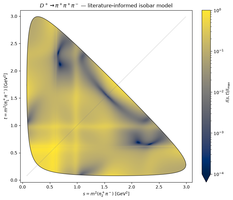
The 1000 × 1000 regular grid avoids Monte Carlo fluctuations and resolves the narrow \(\omega(782)\) contribution. The color is the coherent intensity divided by its maximum on this grid, on a logarithmic scale; it is not a normalized probability density or a measured event count. The two axes distinguish the otherwise identical positive pions. Reflection about \(s=t\) must leave the density unchanged.

../_images/f9b404b2068ccac0102288720b4028664d945eaa31362a96d7ea00bd2a1b33c7.png

The \(\rho(770)\), \(f_0(980)\), and \(f_2(1270)\) bands now have strengths informed by measured component ratios. The heavier states contribute broad structures and interference; their presence does not imply separate visible bands. The small \(\omega(782)\) contribution is concentrated near the \(\rho(770)\) band. The intensity remains symmetric under exchange of the positive pions.